
Processing data with pandas II#
Attention
Finnish university students are encouraged to use the CSC Noppe platform.
![]()
Note
We do not recommended using Binder for this lesson.
This week we will continue developing our skills using pandas to process real data.
Motivation#
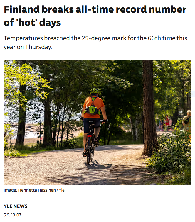
Source: https://yle.fi/a/74-20109657
Finland’s record for the largest number of ‘hot’ days was broken in summer 2024 after temperatures breached the official ‘heatwave’ threshold of 25 degrees Celsius more than 66 times this year. The previous record of 65 hot days was reached in 2002, according to Finnish Meteorological Institute (FMI) statistics Source: YLE.
In this lesson, we will use our data manipulation and analysis skills to analyze weather data, and investigate how hot this summer has been in general in Helsinki and whether this breaking record is valid for several other cities across Finland (Helsinki, Oulu, Lappeenranta, Porvoo, Rovaniemi, and Turku).
Along the way we will cover a number of useful techniques in pandas including:
renaming columns
iterating data frame rows and applying functions
data aggregation
repeating the analysis task for several input files
Input data#
In the lesson this week we are using weather observation data from the Finnish Meteorological Institute. You will be working with temperature data recorded in Helsinki (Kumpula), Lappeenranta (airport), Oulu (Vihreäsaari harbor), Porvoo (Emäsalo), Rovaniemi (railway stattion), and Turku (Rajakari) between June 1st and August 31st 2024.
Downloading the data#
If you are using the CSC Noppe environment, there is no need to download the data manually. The data can be found in the data directory.
However, if you are working in another environment or if you are curious, the data is easily downloadable from the Finnish Meteorological Institute’s open data portal.
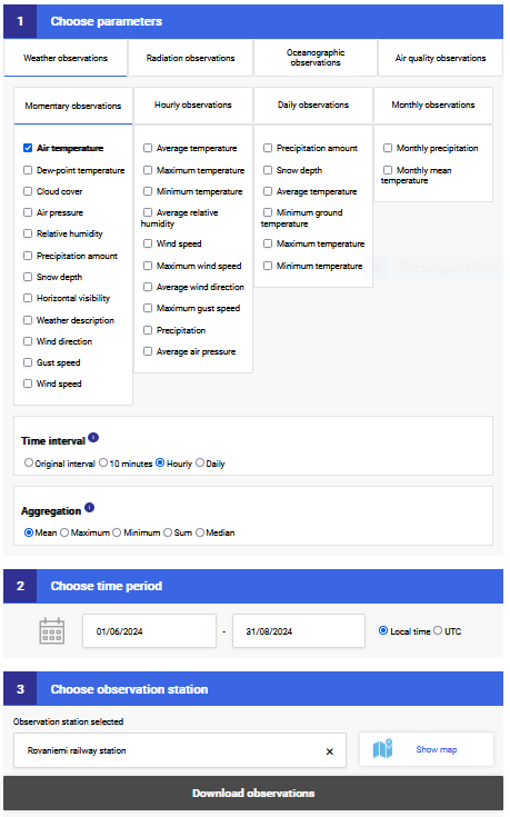
Source: FMI Open Data Portal
Simply choose the parameters you want in your dataset (for this lesson: Air temperature), select the correct time interval (for this lesson: Hourly), choose the aggregation method (Mean), set the time period (1.6.2024 - 31.8.2024), and select the observation station. You can then download the data in various formats. In this lesson we will use CSV files downloaded from the portal.
For this lesson, we are accessing the files from the data directory. For simplicity, the CSV files have been renamed as follows:
Helsinki_Kumpula.csv
Lappeenranta_airport.csv
Oulu_harbour.csv
Porvoo_Emäsalo.csv
Rovaniemi_station.csv
Turku_Rajakari.csv
Now you should be all set to proceed with the lesson!
About the data#
The CSV files have the following structure:
Observation station,Year,Month,Day,Time [Local time],Air temperature mean [°C],Relative humidity mean [%],Gust speed mean [m/s]
Helsinki Kumpula,2024,6,1,00:00,19.3,69.6,1.9
As you can see, the columns are comma-separated. Below is a snippet showing the first row of data from the Helsinki Kumpula observation station:
Observation station |
Year |
Month |
Day |
Time [Local time] |
Air temperature mean [°C] |
Relative humidity mean [%] |
Gust speed mean [m/s] |
|---|---|---|---|---|---|---|---|
Helsinki Kumpula |
2024 |
6 |
1 |
00:00 |
19.3 |
69.6 |
1.9 |
The column names are rather self-explanatory. Here’s a breakdown of what each column contains:
Observation station: The name of the weather station where the measurements were recorded (e.g., Helsinki Kumpula).
Year: The year in which the data was recorded.
Month: The month in which the data was recorded, represented numerically (e.g., 6 for June).
Day: The specific day of the month on which the data was recorded.
Time [Local time]: The time at which the air temperature and other variables were measured, expressed in local time using a 24-hour format.
Air temperature mean [°C]: The mean air temperature recorded at the given time, measured in degrees Celsius.
Relative humidity mean [%]: The average relative humidity at the given time, measured as a percentage.
Gust speed mean [m/s]: The mean wind gust speed at the given time, measured in meters per second.
We will develop our analysis workflow using data from a single station. Then, we will repeat the same process for all the stations.
Reading the data#
In order to get started, let’s first import pandas.
import pandas as pd
At this point, we can already have a quick look at the data file Helsinki_Kumpula.csv and how it is structured.
# Define relative path to the file
fp = r"data/Helsinki_Kumpula.csv"
# Read data and specify the "-" character for NoData values
data = pd.read_csv(fp, na_values=["-"])
Handling No Data Values
The data file from Helsinki does not contain any missing or “No Data” values. However, it is common in many datasets (including others we will use later in this lesson) to encounter missing data. These missing values can be handled or represented in various ways depending on the data source. For instance, they could be encoded as arbitrary values like -9999, or through special symbols such as varying numbers of asterisks *. It’s important to inspect your dataset or review the metadata to be aware of how missing values are represented. This ensures that missing data is correctly interpreted during analysis.
When reading data files with pandas, we can use the na_values parameter to specify a list of values that should be treated as missing. For example, if we had a data file in which missing values were represented by varying numbers of * characters, we could instruct pandas to recognize these as NaN by passing the appropriate list to the na_values parameter (e.g., na_values=['*', '**', '***', '****', '*****', '******']). In addition, if the values were separated by varying numbers of spaces rather than commas we could use the parameter delim_whitespace=True. In that case, the data would be read as shown below.
data = pd.read_csv(
    'datafile.csv', delim_whitespace=True, na_values=["*", "**", "***", "****", "*****", "******"]
)
Let’s see how the data looks by printing the first five rows with the .head() function:
data.head()
| Observation station | Year | Month | Day | Time [Local time] | Air temperature mean [°C] | Relative humidity mean [%] | Gust speed mean [m/s] | |
|---|---|---|---|---|---|---|---|---|
| 0 | Helsinki Kumpula | 2024 | 6 | 1 | 00:00 | 19.3 | 69.6 | 1.9 |
| 1 | Helsinki Kumpula | 2024 | 6 | 1 | 01:00 | 18.9 | 72.5 | 2.7 |
| 2 | Helsinki Kumpula | 2024 | 6 | 1 | 02:00 | 19.7 | 67.4 | 4.3 |
| 3 | Helsinki Kumpula | 2024 | 6 | 1 | 03:00 | 19.4 | 69.2 | 5.4 |
| 4 | Helsinki Kumpula | 2024 | 6 | 1 | 04:00 | 18.5 | 73.6 | 4.5 |
All seems ok. However, we likely won’t be needing all of the columns for detecting warm temperatures. We can check all column names by running data.columns:
data.columns
Index(['Observation station', 'Year', 'Month', 'Day', 'Time [Local time]',
       'Air temperature mean [°C]', 'Relative humidity mean [%]',
       'Gust speed mean [m/s]'],
      dtype='object')
Reading in the data once again#
This time, we will read in only the columns using the usecols parameter. Let’s read in the data again but this time without Relative humidity mean [%] and Gust speed mean [m/s], which would not be useful for our analysis.
# Read in only selected columns
data = pd.read_csv(
    fp,
    usecols=['Observation station', 'Year', 'Month', 'Day','Time [Local time]', 'Air temperature mean [°C]'])

# Check the dataframe
data.head()
| Observation station | Year | Month | Day | Time [Local time] | Air temperature mean [°C] | |
|---|---|---|---|---|---|---|
| 0 | Helsinki Kumpula | 2024 | 6 | 1 | 00:00 | 19.3 |
| 1 | Helsinki Kumpula | 2024 | 6 | 1 | 01:00 | 18.9 |
| 2 | Helsinki Kumpula | 2024 | 6 | 1 | 02:00 | 19.7 |
| 3 | Helsinki Kumpula | 2024 | 6 | 1 | 03:00 | 19.4 |
| 4 | Helsinki Kumpula | 2024 | 6 | 1 | 04:00 | 18.5 |
Renaming columns#
As we saw above, some of the column names are a bit too long. Luckily, it is easy to alter labels in a pandas DataFrame using the .rename() function. In order to change the column names, we need to tell pandas how we want to rename the columns using a dictionary that lists old and new column names
Let’s first check again the current column names in our DataFrame.
data.columns
Index(['Observation station', 'Year', 'Month', 'Day', 'Time [Local time]',
       'Air temperature mean [°C]'],
      dtype='object')
We can define the new column names using a dictionary where we list key: value pairs, in which the original column name (the one which will be replaced) is the key and the new column name is the value.
Dictionaries
A dictionary is a specific type of data structure in Python for storing key-value pairs. In this course, we will use dictionaries mainly when renaming columns in a pandas DataFrame, but dictionaries are useful for many different purposes! For more information about Python dictionaries, check out this tutorial.
Let’s change the following:
Observation stationtoSTATIONTime [Local time]toTIMEAir temperature mean [°C]toTEMP
# Create the dictionary with old and new names
new_names = {"Observation station": "STATION", "Time [Local time]": "TIME", "Air temperature mean [°C]": "TEMP"}

# Let's see what the variable new_names look like
new_names
{'Observation station': 'STATION',
 'Time [Local time]': 'TIME',
 'Air temperature mean [°C]': 'TEMP'}
# Check the data type of the new_names variable
type(new_names)
dict
From above we can see that we have successfully created a new dictionary.
Now we can change the column names by passing that dictionary using the parameter columns in the .rename() function:
# Rename the columns
data = data.rename(columns=new_names)

# Print the new columns
print(data.columns)
Index(['STATION', 'Year', 'Month', 'Day', 'TIME', 'TEMP'], dtype='object')
Perfect, now our column names are more concise.
Check your understanding#
The temperature values in our data files are in degrees Celcius. As you might guess, we will soon convert these temperatures in to degrees Fahrenheit. In order to avoid confusion with the columns, let’s rename the column TEMP to TEMP_C.
Show code cell content
# Solution
# Create the dictionary with old and new names
new_names = {"TEMP": "TEMP_C"}

# Rename the columns
data = data.rename(columns=new_names)

# Check the output
data.head()
| STATION | Year | Month | Day | TIME | TEMP_C | |
|---|---|---|---|---|---|---|
| 0 | Helsinki Kumpula | 2024 | 6 | 1 | 00:00 | 19.3 |
| 1 | Helsinki Kumpula | 2024 | 6 | 1 | 01:00 | 18.9 |
| 2 | Helsinki Kumpula | 2024 | 6 | 1 | 02:00 | 19.7 |
| 3 | Helsinki Kumpula | 2024 | 6 | 1 | 03:00 | 19.4 |
| 4 | Helsinki Kumpula | 2024 | 6 | 1 | 04:00 | 18.5 |
Data properties#
As we learned last week, it’s always a good idea to check basic properties of the input data before proceeding with the data analysis. Let’s check the:
Number of rows and columns
data.shape
(2208, 6)
Top and bottom rows
data.head()
| STATION | Year | Month | Day | TIME | TEMP_C | |
|---|---|---|---|---|---|---|
| 0 | Helsinki Kumpula | 2024 | 6 | 1 | 00:00 | 19.3 |
| 1 | Helsinki Kumpula | 2024 | 6 | 1 | 01:00 | 18.9 |
| 2 | Helsinki Kumpula | 2024 | 6 | 1 | 02:00 | 19.7 |
| 3 | Helsinki Kumpula | 2024 | 6 | 1 | 03:00 | 19.4 |
| 4 | Helsinki Kumpula | 2024 | 6 | 1 | 04:00 | 18.5 |
data.tail()
| STATION | Year | Month | Day | TIME | TEMP_C | |
|---|---|---|---|---|---|---|
| 2203 | Helsinki Kumpula | 2024 | 8 | 31 | 19:00 | 16.9 |
| 2204 | Helsinki Kumpula | 2024 | 8 | 31 | 20:00 | 15.6 |
| 2205 | Helsinki Kumpula | 2024 | 8 | 31 | 21:00 | 15.0 |
| 2206 | Helsinki Kumpula | 2024 | 8 | 31 | 22:00 | 14.4 |
| 2207 | Helsinki Kumpula | 2024 | 8 | 31 | 23:00 | 13.7 |
Data types of the columns
data.dtypes
STATION     object
Year         int64
Month        int64
Day          int64
TIME        object
TEMP_C     float64
dtype: object
Descriptive statistics
data.describe()
| Year | Month | Day | TEMP_C | |
|---|---|---|---|---|
| count | 2208.0 | 2208.000000 | 2208.000000 | 2208.000000 |
| mean | 2024.0 | 7.010870 | 15.836957 | 18.428895 |
| std | 0.0 | 0.814387 | 8.856232 | 3.455590 |
| min | 2024.0 | 6.000000 | 1.000000 | 8.300000 |
| 25% | 2024.0 | 6.000000 | 8.000000 | 16.000000 |
| 50% | 2024.0 | 7.000000 | 16.000000 | 18.400000 |
| 75% | 2024.0 | 8.000000 | 23.250000 | 20.900000 |
| max | 2024.0 | 8.000000 | 31.000000 | 27.300000 |
Using your own functions in pandas#
Now it’s again time to convert temperatures! Yes, we have already done this many times before, but this time we will learn how to apply our own functions to data in a pandas DataFrame.
First, we will define a function for the temperature conversion, and then we will apply this function for each Celsius value on each row of the DataFrame. The output celsius values will be stored in a new column called TEMP_F.
To begin we will see how we can apply the function row-by-row using a for loop and then we will learn how to apply the function to all rows more efficiently all at once.
Defining the function#
For both of these approaches, we first need to define our function to convert temperature from Celsius to Fahrenheit.
def celsius_to_fahr(temp_celsius):
    """Converts temperatures from Celsius to Fahrenheit.

    Parameters
    ----------

    temp_celsius: int | float
        Input temperature in Celsius (should be a number)

    Returns
    -------

    Temperature in Fahrenheit (float)
    """

    # Convert the Celsius into Fahrenheit
    converted_temp = (temp_celsius * 1.8) + 32

    return converted_temp
To make sure everything is working properly, let’s test the function with a known value.
celsius_to_fahr(0)
32.0
Let’s also print out the first rows of our data frame to see our input data before further processing.
data.head()
| STATION | Year | Month | Day | TIME | TEMP_C | |
|---|---|---|---|---|---|---|
| 0 | Helsinki Kumpula | 2024 | 6 | 1 | 00:00 | 19.3 |
| 1 | Helsinki Kumpula | 2024 | 6 | 1 | 01:00 | 18.9 |
| 2 | Helsinki Kumpula | 2024 | 6 | 1 | 02:00 | 19.7 |
| 3 | Helsinki Kumpula | 2024 | 6 | 1 | 03:00 | 19.4 |
| 4 | Helsinki Kumpula | 2024 | 6 | 1 | 04:00 | 18.5 |
Iterating over rows#
We can use the function one row at a time using a for loop and the .iterrows() method. This will allow us to repeat a given process for each row in a pandas DataFrame. Please note that iterating over rows is a rather inefficient approach, but it is still useful to understand the logic behind the iteration.
When using the .iterrows() method it is important to understand that .iterrows() accesses not only the values of one row, but also the index of the row as well.
Let’s start with a simple for loop that goes through each row in our DataFrame.
Note
We use single quotes to select the column TEMP_C of the row in the example below. This is because using double quotes would result in a SyntaxError since Python would interpret this as the end of the string for the print() function.
# Iterate over the rows
for idx, row in data.iterrows():

    # Print the index value
    print(f"Index: {idx}")

    # Print the row
    print(f"Temp C: {row['TEMP_C']}\n")

    break
Index: 0
Temp C: 19.3
Breaking a loop
When developing code in a for loop, you do not always need to go through the entire loop in order to test things out.
The break statement in Python terminates the current loop whereever it is placed and we can use it here just to check out the values on the first row (based on the first iteration in the for loop.
This can be helpful when working with a large data file or dataset, because you might not want to print thousands of values to the screen!
For more information, check out this tutorial.
We can see that the idx variable indeed contains the index value at position 0 (the first row) and the row variable contains all the data from that given row stored as a pandas Series.
Let’s now create an empty column TEMP_F for the Celsius temperatures and update the values in that column using the celsius_to_fahr function we defined earlier.
# Create an empty float column for the output values
data["TEMP_F"] = 0.0

# Iterate over the rows
for idx, row in data.iterrows():

    # Convert the Fahrenheit to Celsius
    temp_fahr = celsius_to_fahr(row["TEMP_C"])

    # Update the value of 'Celsius' column with the converted value
    data.at[idx, "TEMP_F"] = temp_fahr
Reminder: .at[] or .loc[]?
Here, you could also use data.loc[idx, new_column] = temp_fahr to achieve the same result.
If you only need to access a single value in a DataFrame, DataFrame.at[] is faster than DataFrame.loc[], which is designed for accessing groups of rows and columns.
Finally, let’s see how our DataFrame looks after the calculations above.
data.head()
| STATION | Year | Month | Day | TIME | TEMP_C | TEMP_F | |
|---|---|---|---|---|---|---|---|
| 0 | Helsinki Kumpula | 2024 | 6 | 1 | 00:00 | 19.3 | 66.74 |
| 1 | Helsinki Kumpula | 2024 | 6 | 1 | 01:00 | 18.9 | 66.02 |
| 2 | Helsinki Kumpula | 2024 | 6 | 1 | 02:00 | 19.7 | 67.46 |
| 3 | Helsinki Kumpula | 2024 | 6 | 1 | 03:00 | 19.4 | 66.92 |
| 4 | Helsinki Kumpula | 2024 | 6 | 1 | 04:00 | 18.5 | 65.30 |
Applying the function#
Pandas DataFrames and Series have a dedicated method .apply() for applying functions on columns (or rows!). When using .apply(), we pass the function name (without parentheses!) as an argument to the .apply() method. Let’s start by applying the function to the TEMP_C column, which contains the temperature values in degrees Celsius.
data["TEMP_C"].apply(celsius_to_fahr)
0       66.74
1       66.02
2       67.46
3       66.92
4       65.30
        ...
2203    62.42
2204    60.08
2205    59.00
2206    57.92
2207    56.66
Name: TEMP_C, Length: 2208, dtype: float64
The results look logical, so it seems safe to store them permanently in the TEMP_F column (overwriting the old values).
data["TEMP_F"] = data["TEMP_C"].apply(celsius_to_fahr)
Note
We can also apply the conversion function to multiple columns simultaneously while reordering the DataFrame. For instance, if our dataset contained three temperature columns (TEMP, MIN, and MAX), we could perform the conversion and reorganize the columns in one step, as shown below.
data[["TEMP", "MIN", "MAX"]].apply(celsius_to_fahr)
You might also notice that our conversion function would also allow us to pass one column or the entire DataFrame as a parameter (e.g., celsius_to_fahrs(data["TEMP_C"])). However, the code is perhaps easier to follow when using the .apply() method.
Let’s now take a look at the DataFrame contents.
data.head(10)
| STATION | Year | Month | Day | TIME | TEMP_C | TEMP_F | |
|---|---|---|---|---|---|---|---|
| 0 | Helsinki Kumpula | 2024 | 6 | 1 | 00:00 | 19.3 | 66.74 |
| 1 | Helsinki Kumpula | 2024 | 6 | 1 | 01:00 | 18.9 | 66.02 |
| 2 | Helsinki Kumpula | 2024 | 6 | 1 | 02:00 | 19.7 | 67.46 |
| 3 | Helsinki Kumpula | 2024 | 6 | 1 | 03:00 | 19.4 | 66.92 |
| 4 | Helsinki Kumpula | 2024 | 6 | 1 | 04:00 | 18.5 | 65.30 |
| 5 | Helsinki Kumpula | 2024 | 6 | 1 | 05:00 | 18.5 | 65.30 |
| 6 | Helsinki Kumpula | 2024 | 6 | 1 | 06:00 | 18.4 | 65.12 |
| 7 | Helsinki Kumpula | 2024 | 6 | 1 | 07:00 | 20.2 | 68.36 |
| 8 | Helsinki Kumpula | 2024 | 6 | 1 | 08:00 | 21.6 | 70.88 |
| 9 | Helsinki Kumpula | 2024 | 6 | 1 | 09:00 | 23.1 | 73.58 |
Should I use .iterrows() or .apply()?
We are teaching the .iterrows() method because it helps you to understand the structure of a DataFrame and the process of looping through DataFrame rows. However, using .apply() is often far more efficient in terms of execution time.
At this point, the most important thing is that you understand what happens when you are modifying the values in a pandas DataFrame. When doing the course exercises, either of these approaches is ok!
Parsing dates#
As part of this lesson, we want to group our data by day and calculate the average daily temperatures. Currently, we have separate columns storing information on the year, month, and day. Since our data is from the summer of a single year (2024), we do not need to include the year in our grouping. However, we do need to use the information from the month and day for our analysis.
Let’s start by looking at the contents of these columns and their data type:
data["Month"].head(10)
0    6
1    6
2    6
3    6
4    6
5    6
6    6
7    6
8    6
9    6
Name: Month, dtype: int64
data["Day"].tail(10)
2198    31
2199    31
2200    31
2201    31
2202    31
2203    31
2204    31
2205    31
2206    31
2207    31
Name: Day, dtype: int64
The Month and Day columns contain integers. And as evident by the column TIME, several observations are made per day (every hour). We can already see the data types above, but we can check them again using dtypes
data["Month"].dtypes
dtype('int64')
The information in this column is stored as integer values.
We now want to aggregate the data on a daily level, and in order to do so we need to “label” each row of data based on the month and day when the record was observed. In order to do this, we need to somehow aggregate the information for month and day for each row.
We can create these “labels” by making a new column containing information about the month and day.
Before taking that step, hwever, we should first convert the contents in the Month and Day columns to character strings in two new columns.
# Convert to string
data["MONTH_STR"] = data["Month"].astype(str)
data["DAY_STR"] = data["Day"].astype(str)
Now that we have converted the Month and Day data into character strings, the next step is to combine the information from the MONTH_STR and DAY_STR columns into a new column called MONTH_DAY. We will use this format MM-DD.
By applying the .str.zfill(2) method to the DAY_STR and MONTH_STR columns, we ensure that they always have two digits, even when the values are less than 10. This guarantees that the final format is always consistent.
# Combine the two strings
data["MONTH_DAY"] = data["MONTH_STR"].str.zfill(2) + "-" + data["DAY_STR"].str.zfill(2)

# Let's see what we have
data.head()
| STATION | Year | Month | Day | TIME | TEMP_C | TEMP_F | MONTH_STR | DAY_STR | MONTH_DAY | |
|---|---|---|---|---|---|---|---|---|---|---|
| 0 | Helsinki Kumpula | 2024 | 6 | 1 | 00:00 | 19.3 | 66.74 | 6 | 1 | 06-01 |
| 1 | Helsinki Kumpula | 2024 | 6 | 1 | 01:00 | 18.9 | 66.02 | 6 | 1 | 06-01 |
| 2 | Helsinki Kumpula | 2024 | 6 | 1 | 02:00 | 19.7 | 67.46 | 6 | 1 | 06-01 |
| 3 | Helsinki Kumpula | 2024 | 6 | 1 | 03:00 | 19.4 | 66.92 | 6 | 1 | 06-01 |
| 4 | Helsinki Kumpula | 2024 | 6 | 1 | 04:00 | 18.5 | 65.30 | 6 | 1 | 06-01 |
Nice! Now we have “labeled” the rows based on information about date, but only including the month and day in the labels.
String slicing
Date and time data can come in various formats. In some cases, your data may contain a long integer or string representing the date and time. For example, “201910012350” could represent 23:50 on the 1st of October, 2019. In such cases, it is useful to first convert the values to a string (as they may initially be rendered as integers) and then use the pandas.Series.str.slice() method. For example, from the string “201910012350”, you can extract the year and month and write them to a new column YEAR_MONTH as follows:
data["YEAR_MONTH"] = data["TIME_STR"].str.slice(start=0, stop=6)
Datetime (optional)#
In pandas, we can convert date and time information into a specialized data type called datetime using the pandas.to_datetime() function. This allows for more efficient date and time manipulations.
To start, we can create a DATE_STR column by concatenating the Year, Month, and Day columns into a single string in the format YYYYMMDD. We will again apply the .str.zfill(2) method to the MONTH_STR and DAY_STR columns to ensure the formatting is consistent for all dates.
data["YEAR_STR"] = data["Year"].astype(str)
# Combine the three strings
data["DATE_STR"] = data["YEAR_STR"] +  data["MONTH_STR"].str.zfill(2) + data["DAY_STR"].str.zfill(2)
data.head()
| STATION | Year | Month | Day | TIME | TEMP_C | TEMP_F | MONTH_STR | DAY_STR | MONTH_DAY | YEAR_STR | DATE_STR | |
|---|---|---|---|---|---|---|---|---|---|---|---|---|
| 0 | Helsinki Kumpula | 2024 | 6 | 1 | 00:00 | 19.3 | 66.74 | 6 | 1 | 06-01 | 2024 | 20240601 |
| 1 | Helsinki Kumpula | 2024 | 6 | 1 | 01:00 | 18.9 | 66.02 | 6 | 1 | 06-01 | 2024 | 20240601 |
| 2 | Helsinki Kumpula | 2024 | 6 | 1 | 02:00 | 19.7 | 67.46 | 6 | 1 | 06-01 | 2024 | 20240601 |
| 3 | Helsinki Kumpula | 2024 | 6 | 1 | 03:00 | 19.4 | 66.92 | 6 | 1 | 06-01 | 2024 | 20240601 |
| 4 | Helsinki Kumpula | 2024 | 6 | 1 | 04:00 | 18.5 | 65.30 | 6 | 1 | 06-01 | 2024 | 20240601 |
# Convert character strings to datetime
data["DATE"] = pd.to_datetime(data["DATE_STR"])
# Check the output
data["DATE"].head()
0   2024-06-01
1   2024-06-01
2   2024-06-01
3   2024-06-01
4   2024-06-01
Name: DATE, dtype: datetime64[ns]
Pandas Series datetime properties
There are several methods available for accessing information about the properties of datetime values. You can read more about datetime properties from the pandas documentation.
With the new DATE column, we can now extract different time units using the pandas.Series.dt accessor.
data["DATE"].dt.year
0       2024
1       2024
2       2024
3       2024
4       2024
        ...
2203    2024
2204    2024
2205    2024
2206    2024
2207    2024
Name: DATE, Length: 2208, dtype: int32
data["DATE"].dt.month
0       6
1       6
2       6
3       6
4       6
       ..
2203    8
2204    8
2205    8
2206    8
2207    8
Name: DATE, Length: 2208, dtype: int32
We can also combine the datetime functionalities with other methods from pandas. For example, we can check the number of unique months in our input data:
data["DATE"].dt.month.nunique()
3
For the final analysis, we need combined information of the month and day. Here is another way we could achieve this:
# Extract month and day from the full date (as a string in 'MM-DD' format)
data["MONTH_DAY_DT"] = data["DATE"].dt.strftime("%m-%d")
Default Year Behavior in pd.to_datetime()
When using pd.to_datetime() with only month (%m) and day (%d) in the format string, pandas defaults to using the year 1900. This behavior occurs because the datetime module requires a full date, including a year, to function properly. Without a specified year, pandas fills in the year as 1900.
If you need to represent just the month and day without the year, like we do here, we can treat the values as strings using dt.strftime("%m-%d"). This way, we avoid the default year issue.
Alternatively, if you plan to perform date-based operations, you should retain the full date and simply ignore the year in your calculations.
data["MONTH_DAY_DT"]
0       06-01
1       06-01
2       06-01
3       06-01
4       06-01
        ...
2203    08-31
2204    08-31
2205    08-31
2206    08-31
2207    08-31
Name: MONTH_DAY_DT, Length: 2208, dtype: object
Now we have a unique label for each DAY as a datetime object which is the same as what we made ealier without using datetime.
data["MONTH_DAY_DT"] == data["MONTH_DAY"]
0       True
1       True
2       True
3       True
4       True
        ...
2203    True
2204    True
2205    True
2206    True
2207    True
Length: 2208, dtype: bool
Aggregating data in pandas by grouping#
Here, we will learn how to use pandas.DataFrame.groupby(), which is a handy method for combining large amounts of data and computing statistics for subgroups.
In our case, we will use the .groupby() method to calculate average temperatures for each month in three steps:
Grouping the data based on the month and day
Calculating the average for each day (each group)
Storing those values into a new DataFrame called
daily_data
Before we start grouping the data, let’s once again see what our data looks like.
print(f"number of rows: {len(data)}")
number of rows: 2208
data.head()
| STATION | Year | Month | Day | TIME | TEMP_C | TEMP_F | MONTH_STR | DAY_STR | MONTH_DAY | YEAR_STR | DATE_STR | DATE | MONTH_DAY_DT | |
|---|---|---|---|---|---|---|---|---|---|---|---|---|---|---|
| 0 | Helsinki Kumpula | 2024 | 6 | 1 | 00:00 | 19.3 | 66.74 | 6 | 1 | 06-01 | 2024 | 20240601 | 2024-06-01 | 06-01 |
| 1 | Helsinki Kumpula | 2024 | 6 | 1 | 01:00 | 18.9 | 66.02 | 6 | 1 | 06-01 | 2024 | 20240601 | 2024-06-01 | 06-01 |
| 2 | Helsinki Kumpula | 2024 | 6 | 1 | 02:00 | 19.7 | 67.46 | 6 | 1 | 06-01 | 2024 | 20240601 | 2024-06-01 | 06-01 |
| 3 | Helsinki Kumpula | 2024 | 6 | 1 | 03:00 | 19.4 | 66.92 | 6 | 1 | 06-01 | 2024 | 20240601 | 2024-06-01 | 06-01 |
| 4 | Helsinki Kumpula | 2024 | 6 | 1 | 04:00 | 18.5 | 65.30 | 6 | 1 | 06-01 | 2024 | 20240601 | 2024-06-01 | 06-01 |
We have quite a few rows of weather data, and several observations per day. Our goal is to create an aggreated data frame that would have only one row per day.
To condense our data to daily average values we can group our data based on the unique month and day combinations.
grouped = data.groupby("MONTH_DAY")
Note
It is also possible to create combinations of months and days on the fly when grouping the data:
# Group the data
grouped = data.groupby(['Month', 'Day'])
Now, let’s explore the new variable grouped.
type(grouped)
pandas.core.groupby.generic.DataFrameGroupBy
len(grouped)
92
We have a new object with type DataFrameGroupBy with 92 groups. In order to understand what just happened, let’s also check the number of unique month and day combinations in our data.
data["MONTH_DAY"].nunique()
92
Length of the grouped object should be the same as the number of unique values in the column we used for grouping. For each unique value, there is a group of data. This makes sense, as we have 92 days from first of June to the end of August.
Let’s explore our grouped data even further.
We can check the “names” of each group.
grouped.groups.keys()
dict_keys(['06-01', '06-02', '06-03', '06-04', '06-05', '06-06', '06-07', '06-08', '06-09', '06-10', '06-11', '06-12', '06-13', '06-14', '06-15', '06-16', '06-17', '06-18', '06-19', '06-20', '06-21', '06-22', '06-23', '06-24', '06-25', '06-26', '06-27', '06-28', '06-29', '06-30', '07-01', '07-02', '07-03', '07-04', '07-05', '07-06', '07-07', '07-08', '07-09', '07-10', '07-11', '07-12', '07-13', '07-14', '07-15', '07-16', '07-17', '07-18', '07-19', '07-20', '07-21', '07-22', '07-23', '07-24', '07-25', '07-26', '07-27', '07-28', '07-29', '07-30', '07-31', '08-01', '08-02', '08-03', '08-04', '08-05', '08-06', '08-07', '08-08', '08-09', '08-10', '08-11', '08-12', '08-13', '08-14', '08-15', '08-16', '08-17', '08-18', '08-19', '08-20', '08-21', '08-22', '08-23', '08-24', '08-25', '08-26', '08-27', '08-28', '08-29', '08-30', '08-31'])
Accessing data for one group#
Let us now check the contents for the group representing July 17th (the name of that group is 07-17). We can get the values of that hour from the grouped object using the .get_group() method.
# Specify a day (as character string)
day = "07-17"

# Select the group
group1 = grouped.get_group(day)
# Let's see what we have
group1
| STATION | Year | Month | Day | TIME | TEMP_C | TEMP_F | MONTH_STR | DAY_STR | MONTH_DAY | YEAR_STR | DATE_STR | DATE | MONTH_DAY_DT | |
|---|---|---|---|---|---|---|---|---|---|---|---|---|---|---|
| 1104 | Helsinki Kumpula | 2024 | 7 | 17 | 00:00 | 20.2 | 68.36 | 7 | 17 | 07-17 | 2024 | 20240717 | 2024-07-17 | 07-17 |
| 1105 | Helsinki Kumpula | 2024 | 7 | 17 | 01:00 | 19.9 | 67.82 | 7 | 17 | 07-17 | 2024 | 20240717 | 2024-07-17 | 07-17 |
| 1106 | Helsinki Kumpula | 2024 | 7 | 17 | 02:00 | 19.7 | 67.46 | 7 | 17 | 07-17 | 2024 | 20240717 | 2024-07-17 | 07-17 |
| 1107 | Helsinki Kumpula | 2024 | 7 | 17 | 03:00 | 19.8 | 67.64 | 7 | 17 | 07-17 | 2024 | 20240717 | 2024-07-17 | 07-17 |
| 1108 | Helsinki Kumpula | 2024 | 7 | 17 | 04:00 | 19.7 | 67.46 | 7 | 17 | 07-17 | 2024 | 20240717 | 2024-07-17 | 07-17 |
| 1109 | Helsinki Kumpula | 2024 | 7 | 17 | 05:00 | 20.3 | 68.54 | 7 | 17 | 07-17 | 2024 | 20240717 | 2024-07-17 | 07-17 |
| 1110 | Helsinki Kumpula | 2024 | 7 | 17 | 06:00 | 20.6 | 69.08 | 7 | 17 | 07-17 | 2024 | 20240717 | 2024-07-17 | 07-17 |
| 1111 | Helsinki Kumpula | 2024 | 7 | 17 | 07:00 | 20.8 | 69.44 | 7 | 17 | 07-17 | 2024 | 20240717 | 2024-07-17 | 07-17 |
| 1112 | Helsinki Kumpula | 2024 | 7 | 17 | 08:00 | 22.0 | 71.60 | 7 | 17 | 07-17 | 2024 | 20240717 | 2024-07-17 | 07-17 |
| 1113 | Helsinki Kumpula | 2024 | 7 | 17 | 09:00 | 21.7 | 71.06 | 7 | 17 | 07-17 | 2024 | 20240717 | 2024-07-17 | 07-17 |
| 1114 | Helsinki Kumpula | 2024 | 7 | 17 | 10:00 | 21.6 | 70.88 | 7 | 17 | 07-17 | 2024 | 20240717 | 2024-07-17 | 07-17 |
| 1115 | Helsinki Kumpula | 2024 | 7 | 17 | 11:00 | 21.7 | 71.06 | 7 | 17 | 07-17 | 2024 | 20240717 | 2024-07-17 | 07-17 |
| 1116 | Helsinki Kumpula | 2024 | 7 | 17 | 12:00 | 21.7 | 71.06 | 7 | 17 | 07-17 | 2024 | 20240717 | 2024-07-17 | 07-17 |
| 1117 | Helsinki Kumpula | 2024 | 7 | 17 | 13:00 | 21.7 | 71.06 | 7 | 17 | 07-17 | 2024 | 20240717 | 2024-07-17 | 07-17 |
| 1118 | Helsinki Kumpula | 2024 | 7 | 17 | 14:00 | 22.6 | 72.68 | 7 | 17 | 07-17 | 2024 | 20240717 | 2024-07-17 | 07-17 |
| 1119 | Helsinki Kumpula | 2024 | 7 | 17 | 15:00 | 22.9 | 73.22 | 7 | 17 | 07-17 | 2024 | 20240717 | 2024-07-17 | 07-17 |
| 1120 | Helsinki Kumpula | 2024 | 7 | 17 | 16:00 | 23.7 | 74.66 | 7 | 17 | 07-17 | 2024 | 20240717 | 2024-07-17 | 07-17 |
| 1121 | Helsinki Kumpula | 2024 | 7 | 17 | 17:00 | 24.2 | 75.56 | 7 | 17 | 07-17 | 2024 | 20240717 | 2024-07-17 | 07-17 |
| 1122 | Helsinki Kumpula | 2024 | 7 | 17 | 18:00 | 23.5 | 74.30 | 7 | 17 | 07-17 | 2024 | 20240717 | 2024-07-17 | 07-17 |
| 1123 | Helsinki Kumpula | 2024 | 7 | 17 | 19:00 | 21.2 | 70.16 | 7 | 17 | 07-17 | 2024 | 20240717 | 2024-07-17 | 07-17 |
| 1124 | Helsinki Kumpula | 2024 | 7 | 17 | 20:00 | 18.8 | 65.84 | 7 | 17 | 07-17 | 2024 | 20240717 | 2024-07-17 | 07-17 |
| 1125 | Helsinki Kumpula | 2024 | 7 | 17 | 21:00 | 18.4 | 65.12 | 7 | 17 | 07-17 | 2024 | 20240717 | 2024-07-17 | 07-17 |
| 1126 | Helsinki Kumpula | 2024 | 7 | 17 | 22:00 | 18.0 | 64.40 | 7 | 17 | 07-17 | 2024 | 20240717 | 2024-07-17 | 07-17 |
| 1127 | Helsinki Kumpula | 2024 | 7 | 17 | 23:00 | 17.9 | 64.22 | 7 | 17 | 07-17 | 2024 | 20240717 | 2024-07-17 | 07-17 |
Ahaa! As we can see, a single group contains a DataFrame with values only for that specific day. Let’s check the data type of this group.
type(group1)
pandas.core.frame.DataFrame
So, as noted above, one group is a pandas DataFrame! This is really useful, because we can now use all the familiar DataFrame methods for calculating statistics, etc. for this specific group. We can, for example, calculate the average values for all variables using the statistical functions that we have seen already (e.g. mean, std, min, max, median, etc.).
Thus, we can get an average temperature for a given day using the .mean() function that we already did during Lesson 5. Let’s calculate the mean for following attributes all at once:
TEMP_CTEMP_F
# Specify the columns that will be part of the calculation
mean_cols = ["TEMP_C", "TEMP_F"]

# Calculate the mean values all at one go
mean_values = group1[mean_cols].mean()

# Let's see what we have
print(mean_values)
TEMP_C    20.941667
TEMP_F    69.695000
dtype: float64
Above, we saw how you can access data from a single group. In order to get information about all groups (all months) we can use a for loop or methods available in the grouped object.
For loops and grouped objects#
When iterating over the groups in our DataFrameGroupBy object it is important to understand that a single group in our DataFrameGroupBy actually contains not only the actual values, but also information about the key that was used to do the grouping. Hence, when iterating over the data we need to assign the key and the values into separate variables.
So, let’s see how we can iterate over the groups and print the key and the data from a single group (again using break to only see what is happening for the first group).
# Iterate over groups
for key, group in grouped:
    # Print key and group
    print(f"Key:\n {key}")
    print(f"\nFirst rows of data in this group:\n {group.head()}")

    # Stop iteration with break command
    break
Key:
 06-01

First rows of data in this group:
             STATION  Year  Month  Day   TIME  TEMP_C  TEMP_F MONTH_STR  \
0  Helsinki Kumpula  2024      6    1  00:00    19.3   66.74         6
1  Helsinki Kumpula  2024      6    1  01:00    18.9   66.02         6
2  Helsinki Kumpula  2024      6    1  02:00    19.7   67.46         6
3  Helsinki Kumpula  2024      6    1  03:00    19.4   66.92         6
4  Helsinki Kumpula  2024      6    1  04:00    18.5   65.30         6

  DAY_STR MONTH_DAY YEAR_STR  DATE_STR       DATE MONTH_DAY_DT
0       1     06-01     2024  20240601 2024-06-01        06-01
1       1     06-01     2024  20240601 2024-06-01        06-01
2       1     06-01     2024  20240601 2024-06-01        06-01
3       1     06-01     2024  20240601 2024-06-01        06-01
4       1     06-01     2024  20240601 2024-06-01        06-01
OK, so from here we can see that the key contains the name of the group MM-DD.
Let’s build on this and see how we can create a DataFrame where we calculate the mean temperatures in Celsius and Fahrenheit. We will repeat some of the earlier steps here so you can see and better understand what is happening.
# Create an empty DataFrame for the aggregated values
daily_data = pd.DataFrame()

# The columns that we want to aggregate
mean_cols = ["TEMP_F", "TEMP_C"]

# Iterate over the groups
for key, group in grouped:

    # Calculate mean
    mean_values = group[mean_cols].mean()

    # Add the ´key´ (i.e. the date+time information) into the aggregated values
    mean_values["MONTH_DAY"] = key

    # Convert the mean_values series to a DataFrame and make it have a row orientation
    row = mean_values.to_frame().transpose()

    # Concatenate the aggregated values into the daily_data DataFrame
    daily_data = pd.concat([daily_data, row], ignore_index=True)
Note
You can find a slightly more efficient approach for this same kind of aggregation in Chapter 3 of the Python for Geographic Data Analysis textbook.
Now, let us see what we have.
print(daily_data)
     TEMP_F     TEMP_C MONTH_DAY
0   71.7575    22.0875     06-01
1   69.6575  20.920833     06-02
2    69.635  20.908333     06-03
3   68.9825  20.545833     06-04
4     65.87  18.816667     06-05
..      ...        ...       ...
87   63.725     17.625     08-27
88   63.605  17.558333     08-28
89   64.025  17.791667     08-29
90    69.23  20.683333     08-30
91  62.4575  16.920833     08-31

[92 rows x 3 columns]
Awesome! Now we have aggregated our data and we have a new DataFrame called daily_data where we have mean values for each day in the data set.
Detecting warm days in July#
Now that we have aggregated our data on daily level, we want to sort our results in order to check which days in July had the warmest temperatures on average. A simple approach is to select all the data rows from July and then group the data and check which group(s) (days in our case) have the highest mean value.
July_days = data[data["Month"] == 7]
Next, we can take a subset of columns that might contain interesting information.
July_days = July_days[["TEMP_F", "TEMP_C", "MONTH_DAY"]]
We can group by month and day.
grouped = July_days.groupby(by="MONTH_DAY")
And then we can calculate the mean for each group.
daily_mean_July = grouped.mean()
daily_mean_July.head()
| TEMP_F | TEMP_C | |
|---|---|---|
| MONTH_DAY | ||
| 07-01 | 66.1250 | 18.958333 |
| 07-02 | 65.4875 | 18.604167 |
| 07-03 | 58.9400 | 14.966667 |
| 07-04 | 62.8175 | 17.120833 |
| 07-05 | 62.3000 | 16.833333 |
Finally, we can sort and check the highest temperature values. We can sort the data frame in a descending order to do this.
daily_mean_July.sort_values(by="TEMP_C", ascending=False).head(10)
| TEMP_F | TEMP_C | |
|---|---|---|
| MONTH_DAY | ||
| 07-26 | 72.8600 | 22.700000 |
| 07-25 | 72.2300 | 22.350000 |
| 07-24 | 72.0275 | 22.237500 |
| 07-23 | 71.9075 | 22.170833 |
| 07-27 | 70.5950 | 21.441667 |
| 07-29 | 70.4900 | 21.383333 |
| 07-22 | 70.3175 | 21.287500 |
| 07-28 | 69.8825 | 21.045833 |
| 07-17 | 69.6950 | 20.941667 |
| 07-13 | 69.6125 | 20.895833 |
So, what were the warmest days in July?
Did we break the record in Helsinki?#
While the average temperature provides a general sense of how warm the days typically are, the news article about record-breaking heat was based on the highest recorded temperature of the day. Now, we will redo the grouping of the data by day for the whole summer, but instead of calculating the mean temperature, we will calculate the maximum recorded temperature for each day.
data.head()
| STATION | Year | Month | Day | TIME | TEMP_C | TEMP_F | MONTH_STR | DAY_STR | MONTH_DAY | YEAR_STR | DATE_STR | DATE | MONTH_DAY_DT | |
|---|---|---|---|---|---|---|---|---|---|---|---|---|---|---|
| 0 | Helsinki Kumpula | 2024 | 6 | 1 | 00:00 | 19.3 | 66.74 | 6 | 1 | 06-01 | 2024 | 20240601 | 2024-06-01 | 06-01 |
| 1 | Helsinki Kumpula | 2024 | 6 | 1 | 01:00 | 18.9 | 66.02 | 6 | 1 | 06-01 | 2024 | 20240601 | 2024-06-01 | 06-01 |
| 2 | Helsinki Kumpula | 2024 | 6 | 1 | 02:00 | 19.7 | 67.46 | 6 | 1 | 06-01 | 2024 | 20240601 | 2024-06-01 | 06-01 |
| 3 | Helsinki Kumpula | 2024 | 6 | 1 | 03:00 | 19.4 | 66.92 | 6 | 1 | 06-01 | 2024 | 20240601 | 2024-06-01 | 06-01 |
| 4 | Helsinki Kumpula | 2024 | 6 | 1 | 04:00 | 18.5 | 65.30 | 6 | 1 | 06-01 | 2024 | 20240601 | 2024-06-01 | 06-01 |
# Select all days and leep only two columns
summer_days = data[["TEMP_C", "MONTH_DAY"]]

# Group data based by days
grouped = summer_days.groupby(by="MONTH_DAY")

# Calculate the daily maximum temperature
daily_max = grouped.max()

# Rename the column TEMP_C to MAX_C for better clarity
daily_max = daily_max.rename(columns={"TEMP_C": "MAX_C"})

# View the first five rows of output data
daily_max.head()
| MAX_C | |
|---|---|
| MONTH_DAY | |
| 06-01 | 26.2 |
| 06-02 | 24.5 |
| 06-03 | 25.7 |
| 06-04 | 24.6 |
| 06-05 | 23.3 |
Now let’s count the number of hot days (>= 25 degrees celsius) in Helsinki and see whether the country record was also broken in Helsinki or not?
# Try it your self
count_hot_days = len(daily_max[daily_max["MAX_C"] >= 25])
print(f"In the summer of 2024, there were {count_hot_days} days with temperatures exceeding 25°C.")
In the summer of 2024, there were 12 days with temperatures exceeding 25°C.
Repeating the data analysis with a larger dataset#
To wrap up today’s lesson, let’s repeat the data analysis steps above for all the available data we have (!). Of course we want to automate this process and not repeate the process for each dataset.
The idea is, that we will repeat the analysis process for each input file using a (rather long) for loop! Here we have all the main analysis steps with some additional output info, all in one long code cell.
At this point we will use the .glob() function from the module glob to list our input files. glob is a handy function for finding files in a directrory that match a given pattern, for example.
import glob
file_list = glob.glob(r"data/*csv")
Note
Note that we’re using the * character as a wildcard, so any file that starts with data/ and ends with csv will be added to the list of files we will iterate over. In our case there are not other data files in this directory. But this can be specifically useful if there are other files in the folder which we do not want to include in the analysis.
print(f"Number of files in the list: {len(file_list)}")
print(file_list)
Number of files in the list: 6
['data/Lappeenranta_airport.csv', 'data/Porvoo_Emäsalo.csv', 'data/Helsinki_Kumpula.csv', 'data/Turku_Rajakari.csv', 'data/Rovaniemi_station.csv', 'data/Oulu_harbour.csv']
Now, you should have all the relevant file names in a list, and we can loop over the list using a for loop.
for fp in file_list:
    print(fp)
data/Lappeenranta_airport.csv
data/Porvoo_Emäsalo.csv
data/Helsinki_Kumpula.csv
data/Turku_Rajakari.csv
data/Rovaniemi_station.csv
data/Oulu_harbour.csv
And here is our for loop to repeat the calculation for all our data from the different stations:
# Repeat the analysis steps for each input file:
for fp in file_list:

    # read the data, some datasets have missing values filled as "-"
    data = pd.read_csv(
        fp,
        usecols=['Observation station', 'Year', 'Month', 'Day','Time [Local time]', 'Air temperature mean [°C]'], na_values=["-"])

    # Create the dictionary with old and new names
    new_names = {"Observation station": "STATION", "Time [Local time]": "TIME", "Air temperature mean [°C]": "TEMP_C"}

    # Rename the columns
    data = data.rename(columns=new_names)

    # Convert to string
    data["MONTH_STR"] = data["Month"].astype(str)
    data["DAY_STR"] = data["Day"].astype(str)

    # Combine the two strings
    data["MONTH_DAY"] = data["MONTH_STR"].str.zfill(2) + "-" + data["DAY_STR"].str.zfill(2)

    # Select all days and leep only two columns
    summer_days = data[["TEMP_C", "MONTH_DAY"]]

    # Group data based by days
    grouped = summer_days.groupby(by="MONTH_DAY")

    # Calculate the daily maximum temperature
    daily_max = grouped.max()

    # Rename the column TEMP_C to MAX_C for better clarity
    daily_max = daily_max.rename(columns={"TEMP_C": "MAX_C"})

    count_hot_days = len(daily_max[daily_max["MAX_C"] >= 25])

    # Extract station name from fp - the part of the string between 'data/' and '.csv'
    station_name = fp.split('\\')[-1].replace('.csv', '')

    print(f"In the summer of 2024, there were {count_hot_days} days with temperatures exceeding 25°C in {station_name}")
    print("\n")
In the summer of 2024, there were 17 days with temperatures exceeding 25°C in data/Lappeenranta_airport


In the summer of 2024, there were 0 days with temperatures exceeding 25°C in data/Porvoo_Emäsalo


In the summer of 2024, there were 12 days with temperatures exceeding 25°C in data/Helsinki_Kumpula


In the summer of 2024, there were 2 days with temperatures exceeding 25°C in data/Turku_Rajakari


In the summer of 2024, there were 12 days with temperatures exceeding 25°C in data/Rovaniemi_station


In the summer of 2024, there were 5 days with temperatures exceeding 25°C in data/Oulu_harbour
So, what can we conclude about record breaking hot days in Summer 2024 in Finland?